Intro

You have all had to implement a moving average algorithm from time-to-time. Moving averages make life easier, especially for mixed-signal applications in which you have a few extra A/D cycles available.

This article is intended for a fixed-point audience; however, the techniques shown can apply to floating point data as well, with slight modifications.

The remainder of the article will assume that the user is working with signed 16-bit numbers, which have a range of -32768 to +32767. This is just for illustration and doesn't in any way impose an upper or lower limit on the technique.

Typical Moving Average

The typical takes some number of elements and averages them, then takes the next group of elements, then averages those and so on. This is simple and highly effective. If you only require a two-element moving average, this is the way to go. If you require a 16-element moving average, then the process of creating a moving average involves:

Saving 16 elements of data, probably in an array (32 bytes of RAM)
Adding all of these elements up
Dividing the elements by 16

We can optimize a couple of these processes. For one, if you create an extra 'accumulator' value, then you can simply add the newest value to it and subtract the oldest value from it instead of adding all elements up.

Additionally, if you make your array length a power of 2, you can 'divide' by simple bit shifting.

RAM Breakdown

Assuming your accumulator is twice the sample width, your RAM usage in this instance is:

32 bytes for your data array
1 byte for your array index counter
4 bytes for your accumulator

For a total of 37 bytes utilized. This won't break the bank on your standard smartphone or x64, but this is nearly half of your RAM on an MSP430!

Cycles Breakdown

1 add operation
1 subtract operation
1 divide/shift operation

Assuming that we are shifting and not dividing, this isn't too bad a penalty to pay for the moving average.

Modified Moving Average

Lets just get right into a bit of pseudocode:

avg_accum += new_sample;

avg_accum =- sample_average;

sample_average = avg_accum >> x;

The above pseudocode is executed on every new sample. The 'accumulator' adds a 'new_sample' and subtracts an 'sample_average' on each run around. The new 'sample_average' is then calculated by shifting the bits by 'x', which will usually be a static value. A higher number creates a stronger filter.

Effectively, this technique works by giving weight to older data by reducing the weight of newer data by the amount shifted, 'x'.

RAM breakdown

4 bytes for the accumulator
2 bytes for the average (it is persistent, cycle-to-cycle)

For a total of 6 bytes.

Cycles Breakdown

1 add operation
1 subtract operation
1 divide/shift operation

Identical to the moving average, so this is a wash.

Comparisons

So lets run these filters through some rudimentary testing through a 16-sample moving average filter and then match that with our 'lean' filter.

Impulse Response

impulse

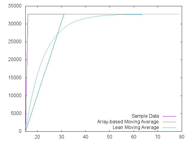
The left-most sample number of the chart is actually a value of '15' at a value of '0' so that the moving average filter could get enough samples to be 'primed'. At sample 16, the sample impulses to 32767 and the filter responses are shown. I realize that a typical moving average filter would not have the phase delay, but that is a choice that I made to ease coding.

The moving average filter will simply average the group of 16 samples until it gets to the maximum, resulting in the linear ramp to maximum shown.

The reader familiar with electronics will note the similarity between the 'lean' response and the exponential response common in RC and RL filters. I don't know if they are actually equivalent, but the resemblance is striking. Perhaps a gifted reader could tackle this question?

We adjusted the shift operation until the plotted response of the two methods were reasonably close and ended up with a shift of '3', which is effectively division by 8.

Random Noise

The impulse response is cool and shows that there is some real filtering going on in the lean version, but what about random data? We took random numbers between 0 and 32767 and ran them through each filter. Lets take a look:

random noise plot

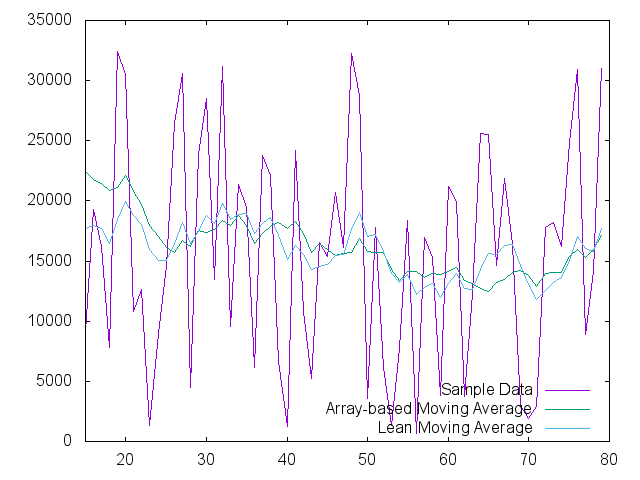
It is clear from the two plots that both datasets demonstrate effective filtering of the random data. There are places in which each seems to work more effectively, but both are holding the value near the 16383 average value.

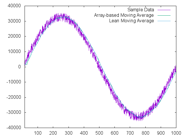
Noisy Waveform

Placing the filters on an actual wave shape will help the reader visualize the effectiveness of the filter as well:

noisy sine plot

Summary

If you are looking for a simple and effective filter for your low-resource project, this is it. Adjustment is simple and, unlike the standard moving average filter, doesn't require any more RAM to keep the older samples.

The filter simulation was run using Python. Source code is on github.