The First Shots are In!

After a few weeks of messing around on-and-off with the curve tracer, we finally have some shots to show that the work has not been for nothing!

The Tool

I took the time to write a small TkInter-based plotting tool. I found a couple of examples out there, but nothing that seemed to fit the bill. I thought of using a framework like PyQt or matplotlib, but I wanted to ensure that the final package was completely compileable and in Python3, so I rolled my own.

Admittedly, the plot tool isn't very good right now, but I suspect that it will get better.

The Screenshots

The plot consists of a grid of dotted lines and solid lines. The solid lines are the '0' of each axis. On the horizontal axis, the scale goes from -5V to 5V. Each dotted crossing represents 1V. On the vertical axis, the scale is:

\(100\Omega \frac{24k\Omega}{2.67k\Omega}\) \(= 100\frac{V}{A} \frac{24}{2.67}\) \(= 899\frac{V}{A}\)

The vertical division is also in Volts, but converting that to current means that the vertical divisions are:

\(\frac{1}{899\frac{V}{A}}\) \(= 1.11\frac{mA}{V}\)

So the vertical divisions represent 1.11mA each, for a full-scale of 5.55mA. Our original intent was to have the gain be "10" rather than "8.99", but you may recall that we didn't have any 10kΩ resistors in the SMT package and changed the ratio slightly. This will be corrected in the next schematic/layout session.

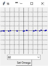
Open Circuit

The first picture is the standard 'open circuit'. The voltage traverses the entire scale while the current remains at 0A.

open circuit

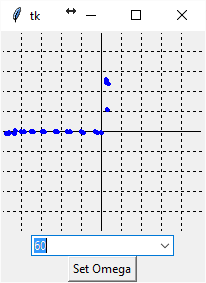
Short Circuit

We connected the leads together and expect that the voltage will be very small and the current will be traverse the vertical range...

short circuit

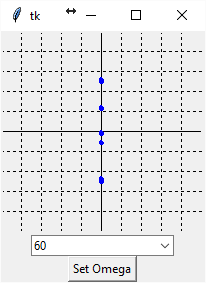
Ok, so the dots are off-putting. I will work on the presentation, but it is working and that is what counts.

Resistor, 100Ω

Next, we try a 100Ω resistor. We expect a 'high' current to flow, but there should be some voltage applied. Note that Ohm's Law is a linear equation, meaning that an ohm of resistance implies a Volts/Amp relationship. Our curve tracer should reflect that since we are looking directly at the Volt-Amp relationship on a resistor. We are actually seeing Ohm's Law in action!

100Ω resistor

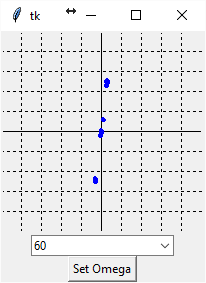
There is a steep slope, but there is definitely a 'lean' to it that wasn't there on a short circuit. Success!

Resistor, 1kΩ

The 1kΩ resistor should have a much lower slope than the 100Ω resistor...

1kΩ resistor

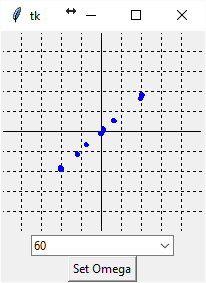
Just as predicted! It seems that things are working.

Capacitor, 10μF

Now, lets introduce a bit of reactance into the equation by throwing a capacitor in the mix. With a capacitor, the current leads the voltage, so we expect an ellipse.

10μF capacitor

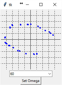
Well, it isn't a perfect ellipse, but - at this point - we know that the concepts are serving us well.

Diode

Finally, one of the most iconic VI curves is that of the diode, which is "open" in one polarity and "short" in the other polarity. We have an MBR1100, which is a Schottky diode.

diode

Perfect!

Next Steps

During this testing, we found a glitch somewhere in the communications channel. We will get all of the tested code from Dispatch working rather than using the implementation that was ad-hoc written here. We will also attempt to firm up the Python library in the process. After that, some solid work on the visuallization and data rate to get more points would probably be in order.

After all of the posts, it is nice to see it coming together!